Hearing is Believing vs. Believing is Hearing: Blind vs. Sighted Listening Tests, and Other Interesting Things 3894 (H-6) Floyd E. Toole and Sean E. Olive Harman International Industries, Inc. Northridge, CA 91329, USA Presented at the 97th Convention 1994 November 10-13 SanFrancisco AuD,O This preprint has been reproduced from the author's advance manuscript, without editing, corrections or consideration by the Review Board. The AES takes no responsibility for the contents. Additional preprints may be obtained by sending request and remittance to the Audio Engineering Society, 60 East 42nd St., New York, New York 10165-2520, USA. Afl rights reserved. Reproduction of thispreprint, or any portion thereof, is not permitted without direct permission from the Journal of the Audio Engineering Society. AN AUDIO ENGINEERING SOCIETY PREPRINT Blind Hearing vs. Sighted is Believing vs. Believing is Hearing: Listening Tests, and Other Interesting Things by Floyd E. Toole and Sean E. Olive Harman International Industries, Inc. Northridge, CA 91329 U.S.A. Although it is taken for granted that many factors influence listeners as they form opinions of sound quality, it is interesting to actually put them to the test, and to assess the strength of the factors. These experiments had several objectives. On the subjective side, they were to determine the extent to which listeners' opinions about loudspeaker sound quality are affected by not seeing (blind tests) and seeing (sighted tests) the loudspeakers being evaluated, to examine the performance of listeners with and without experience in critical listening, and to examine the influence of the sex of the listener. On the product side, the objectives were to evaluate the differences among three high-quality expensive loudspeakers and a high-performance, small, inexpensive system which would serve as an "honesty' check for listeners in the sighted tests. The results contain some reassurances and some surprises. 0 INTRODUCTION Many years of experience with listening tests, conducted under blind and double-blind circumstances have proven their worth and reliability in quantifying subjective responses to several measureable parameters. The results of these psychoacoustic investigations have been repeatable and, with retrospect, the relationships between the subjective and objective domains have been logical [1,2,3]. In properly conducted controlled tests, listeners have been shown to be extremely sensitive to small changes in sound quality. Yet, there continue to be animated arguments about the validity of blind tests. The majority of these apply to the "great debate" issues, related to the question of whether certain differences are audible or not. This paper does not address this debate. All of the differences associated with the subjective evaluations in these experiments were very audible, even to untrained listeners. The question here was: given that certain differences among products are clearly audible, to what extent are listeners' opinions altered when they are aware of the products being listened to? It is probably safe to say that everyone in audio has been involved in "sighted" subjective evaluations at one time or other. It is probably a safe generalization to say that most people in audio think that they can ignore the effects of prior knowledge when they focus on the sounds of the products under examination. Others would argue that it is difficult to impossible not to be biased in some way by expectations. But... have you ever put it to the test? Probably not. Neither had we. Experience is one of those variables among listeners that is very difficult to quantify. For example, musicians are experienced listeners but, is experience in focusing on musical attributes equivalent to that of focusing on timbral and spatial attributes? Some evidence suggests that it is not. Gabrielsson found that musicians who were not also audiophiles, were not especially good judges of sound quality[4]. The famous pianist Glenn Gould came to appreciate the insights of non musicians[5]. Our own tests have confirmed this. So, listeners with different backgrounds could be expected to have differing abilities or preferences in subjective evaluations. This is an enormously broad topic, but we thought that it would be interesting to take a first step towards understanding the importance of this variable. Everyone knows that females have different preferences to males. Right? If so, where is the proof?. Some earlier tests included both male and female participants [6]. In this case, they were all professional sound engineers and producers. In the final analysis, their opinions were indistinguishable from those of their male colleagues. There was one difference, however:, a lower percentage of them had hearing loss so that, as a population, they were more reliable listeners. At the consumer level, there remains the question about sexual bias in listener preferences. We now have some data. The issues addressed in these evaluations are important. They are also not unidimensional Definitive answers must await more data but, in the meantime, it is interesting to have some light shed on the issues. 2 OBJECTIVES · · · · · · These tests had several objectives. On the subjective side they were: to determine the extent to which listeners' opinions about loudspeaker sound quality are affected by not seeing (blind tests) and seeing (sighted tests) the loudspeakers being evaluated, to examine the influence of having experience in critical-listening, and to examine the influence of the sex of the listener. On the product side, the objectives were: to evaluate the differences between two different variations of the same basic loudspeaker system. They employed the same drivers in the same enclosure, but the crossover networks were designed by two different engineers having slightly different opinions about the optimum spectral smoothness and balance. These are high-priced, high-end products. to compare these performances with that of a current audiophile favorite of a comparable price and size. to evaluate a compact, inexpensive, subwoofer/satellite system, and to use it as an "honesty" check for listeners in the sighted tests. Previous tests had shown that, within its power-handling capabilities, it performed in a manner that belied its low price and small size. 3 METHOD So that the results would carry some weight, forty (40) listeners participated in the blind and sighted tests. They were all employees of Ilarman International companies. This means that, in the sighted tests, the listeners had one bias in common: brand loyalty. The effects were tested using male experienced listeners and both male and female inexperienced listeners. In these tests, listeners were considered to be inexperienced if they had no previous experience in controlled listening tests. Other definitions are possible, which might include persons with no critical listening experience whatsoever. The participants were categorized under the following headings. LISTENERS BLIND TESTS Experienced Inexperienced Male 10 10 Female 0 5 Total 10 15 Sex SIGHTED TESTS Experienced Inexperienced 8 4 0 :3 8 !7 Unfortunately, it was not possible to balance all levels within each category. In Experiment 1 different listeners participated in the blind and sighted versions. As a further test, Experiment 2 was conducted, in which the same four experienced listeners participated in both versions. The listening room was typical of a domestic listening situation. In the blind tests, the identities of the loudspeakers were hidden from the listeners with a visually opaque screen made of loudspeaker grille cloth. The grilles were removed from the loudspeakers so that, in effect, the grille cloth hid the entire loudspeaker, not just the drivers. In the sighted tests, the screen was removed and listeners were told the brand name, model number and retail price of each speaker prior to the start of the test. The tests were conducted over a period of 1.5 weeks using a multiple ( 4 loudspeakers at a time) presentation method. The monophonic tests were conducted with the loudspeakers adjusted for equal loudness within 0.5 dB using B -weighted pink noise. Playback levels, which were constant throughout the tests, were set for typical "good listening". They were not intended to explore the power-handling capabilities of the systems. Listeners completed two rounds, in each round giving ratings for four different loudspeakers for each of the 4 different programs. Between rounds, the speaker locations were changed. The order of rounds was randomized among the ten different listening groups. Listeners remained in the same seat locations throughout all tests. Listeners rated the loudspeakers using a 10 point Preference Scale, where higher ratings indicate greater preferences. This is not the same as the Fidelity Scale used in earlier tests by Toole[1]. This scale is designed to accentuate perceived differences between the loudspeakers[7]. The duration of the entire test was about 20-30 minutes. Excerpts from the 4 programs were digitally copied from CD on to a hard-disc, edited into 30 second repeating loops, and then transferred to R-DAT for the test playbacks. 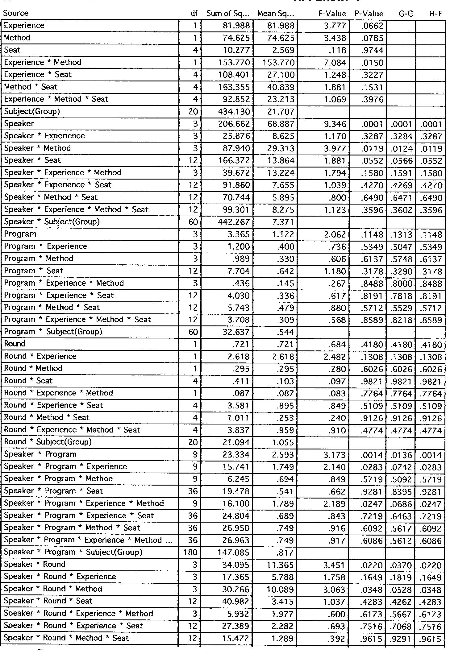The programs used were: ABBREVIATION TC LF 'PS SS PROGRAM Tracy Chapman/Fast Car Little Feat/Let the Good Times Roll Paul Simon/Graceland Full Orchestra/Stars & Stripes 4 RESULTS 4.1 EXPERIMENT ONE The ratings from both experiments were analyzed using a repeatedmeasures analysis of variance (ANOVA). This is an analysis which evaluates the contribution of the individual variables, and the interactions between them, to the variations in listeners' numerical judgments. APPENDIX 1 shows the ANOVA table for each source of variance and their interactions. If the H-F value is <= 0.05 then the source had an effect on the loudspeaker ratings with a probability of 95% that the listener responses did not occur due to chance. "Method" is the variable "blind" vs. "sighted". It is reassuring that the influential factors and interactions are those that one would logically think should modify listener opinions. It is important to note that, in a test of sound quality, not all of the important variables were related to sound. Visual cues had several statistically significant influences. · Speaker (This is a very strong influence, as it should be.) · Speaker * Method (Seeing the products had a strong influence on ratings of the loudspeakers) · Speaker * Seat (Where the listener sat in the room had a strong effect on the ratings. This is an acoustical effect related to the peculiarities of the listening room, and the directional properties of the loudspeakers.) · Speaker * Program (The choice of music affected the ratings. Listeners' tastes in music occasionally are involved here but, much more important, are the facts that (a) musical selections are not all equally good at revealing problems in loudspeakers, and (b) that different recordings have different spectral balances ("voices) which interact with the different "voicings" of the loudspeakers.) · Speaker * Program * Experience (The choice of music affected opinions of experienced listeners differently than those of inexperienced listeners. Some listeners, mainly inexperienced ones, tend to stay with a first impression, and not change it through quite wide variations in program material.) · Speaker * Program * Experience * Method (As above, but seeing the loudspeakers made a difference) · Speaker * Round (The locations of the loudspeakers in the room made a difference to the sound. This is a well known phenomenon. It has been scientifically demonstrated that, in tests involving good and closely rated loudspeakers, the locations of the loudspeakers in the room can be the dominant factor in determining the ratings [8,9].) · Speaker * Round * Method (As above, but seeing the loudspeakers made the differences matter less.) The specifics of these factors are discussed in the following sections. 4.1.1 Loudspeaker Preferences Combining the results of all listeners in all rounds, indicates that models "D" and "G' were slightly to moderately preferred over "S" oald "T', Figure 1. Be careful not to be misled by the scaling of this graph. The total vertical height is less than a third of the 10-point preference scale. In the normal context of listening tests, this is a small range of ratings, indicating a fairly close contest. There were no truly bad loudspeakers here. t_ Z "' o Z Interaction Bar Chart Effect: Speaker Dependent: PreferenceRatings With 95% Confidence error 8 i i 7 bars. i i T 1 I.J.I 1.1.1 1,1,. © ,,, TII Z I.IJ ',j: $ .... G D S T LOUDSPEAKER Figure 1. Combined results of all tests, blind and sighted, showing means of preference ratings for ali listeners. Note that the vertical only a portion of the 0 - 10 preference scale. the cell scale is The results show that the loudspeakers fell into two closely "G" and "D", and "S" and "T". The listeners clearly preferred the the second pair but, within the pairs, the error bars indicate that preference that was statistically important. Remember that these contain a mixture of all tests, sighted and blind. There is more to rated pairs, first pair to they had no results this story. 4.1.2 Effect Position Loudspeaker of Test Method (Blind Versus Sighted) There is now abundant evidence that the listening positions of loudspeakers within the room are significant and room and the influences on listener opinions of loudspeakers. In the blind tests, in which listeners only the sound to rely on, preference ratings were strongly dependent locations of the loudspeakers, Figure 2. Interaction Bar had on the Chart Effect: Speaker * Round * Method Dependent: PreferenceRatings With 95% Confidence error bars. o Z LIJ Z L_J _r LIJ L[ IJ.I _r I II O Z La LOCATION 1 BLIND LOCATION 2 BLIND LOCATION 1 SIGHTED Figure 2 A comparison of results the loudspeaker locations. for the blind LOCATION 2 SIGHTED and sighted tests, for each of In fact, in the blind tests, where opinions were based solely on sound, the location of the loudspeakers in the room had more of an effect in the preferences of these loudspeakers, than the loudspeakers themselves. In location 1, the listeners exhibited no clear preference for any of the four loudspeakers. In location 2, however, there were strong preferences. Obviously, important difference in sound quality were introduced by the position factor. However, in the sighted tests, the ratings were very strongly differentiated, and they did not change appreciably between the two sets of room locations. In other words, in this test, when listeners knew what they were listening to, the opinions were dictated more by the product identity than by the sound. If we isolate the visual and political factors we have the following possible scenario. It is easy to believe that loudspeakers "G' and "D" would be viewed favorably because they were the most expensive, the largest, quite attractive, and they were products of the company that employed the hsteners. Loudspeaker 'T" was slightly smaller, slightly less expensive, a prestige product, but made by a competitor. Loudspeaker "S' was absolutely tiny, relatively inexpensive, and plastic. It was a product of the host company, but could anything that small and cheap be any good? Many listeners in the sighted tests admitted afterwards that before the music even started they believed that loudspeaker "S' would sound inferior, although they admitted its strong performance surprised them. Combining the data from tests in both of the loudspeaker locations, Figure 3 isolates the effect of seeing the products that are being evaluated. The separation of the products into two groups is dear in both results, but the preference of loudspeaker "T' over loudspeaker "S" is evident only in the "sighted" results. Interaction Bar Chart Effect: Speaker * Method Dependent: PreferenceRatings With 95%-Confidence error bars. o Z re W O Z W t'e W tL LU m' I © Z W _r Figure 3 combining BLIND SIGHTED A comparison of listener preferences in blind and sighted tests, the results of tests performed in two loudspea_ker locations. Some of us would like to think that we can ignore visual factors when at opinions of sound quality.., but can we7 An overall effect that is interesting, but not of any real consequence here, is that listeners in the "sighted" tests (both experienced and inexperienced ) used higher ratings compared to listeners in the blind tests, Figure 4. We can speculate that listeners may use higher ratings when they can see the products because they are more confident in their opinions, or they are less concerned about revealing inconsistencies in their judgments, or both. arriving _l_ 8 I I Z W 0 T ill w T l.l. III ell LL 6 © Z w _ I l BLIND Figure 4 by listeners Averaged in blind SIGHTED across all experiments, and sighted tests. a comparison of the ratings used Z [- W :ir r'l 6 o, T ;[i il ij ij [i j[ i, Z w zo '" = u. ILl 7 S !iiiiiiiiiiiiiii[iiiiiiiiiiiii BLIND [] [] Figure listeners T T :iiii!iiiiiii!il!!iiiliil SIGHTED EXPERIENCED LISTENERS INEXPERIENCED LISTENERS 5 A comparison of the ratings in blind and sighted tests used by experienced and inexperienced 4.1.3 The Effect of Listener Experience Separating the listeners by experience, Figure 5, it becomes clear that it is the experienced listeners in the blind tests that caused the strongest differentiation. Experienced listeners used lower ratings than inexperienced listeners in the blind tests but in the sighted tests the difference disappeared. While it is interesting to speculate about why this occurs, the absolute ratings used by listeners are of no consequence to the important result, which is the relative ratings of the products under evaluation. In this it can be clearly stated that the inexperienced male listeners had the same loudspeaker preferences as the experienced male listeners, Figure 6. Interaction Bar Chart Effect: Speaker * Experience * Sex Dependent: PreferenceRatings With 95% Confidence error bars. E_ Z w er tlJ Z LIJ W LI. LLI er O. u. m O Z ila _r EXPERIENCED MALES Figure 6 experience. Loudspeaker 4.1.4 Effect The INEXPERIENCED MALES EXPERIENCED INEXPERIENCED FEMALES FEMALES preferences classified by sex and listening of Sex There is a popular belief that females have different preferences in loudspeakers than males. The folklore is rich with tales of irreconcilable differences between the sexes. Some evidence suggests that other factors may have been involved, such as price, size, style, loudness, purchasing priorities, etc. Here, though, we ignore everything but the sound, and ask the question. Figure 6 shows that the opinions of inexperienced male and inexperienced female listeners (see the two right-hand histograms) are remarkably similar. Viva la similaritY! 4.1.5 The Effect of Listener Location The interactions among loudspeaker, loudspeaker position and listener position are strong and complex. When comparing loudspeakers that are comparably good in terms of timbral accuracy, as these loudspeakers are, one must be aware of these effects ff the results are to be trusted. In these experiments the physical differences in loudspeaker locations between rounds were much smaller than differences between listener locations. Listener location is therefore the stronger variable. Figure 7 shows that front row listeners in seats 1 and 2 had similar loudspeaker preferences, although seat 2 listeners slightly preferred model "D'. Back row listeners (seats 3, 4 and 5) showed differing preferences. t_ Z er LId Z ul er LU i1 UJ ee i [J. © Z w 1/ FRONTROW Figure 8 Loudspeaker preference BACKROW ratings as a function of listener location. It is interesting to look for trends in these data. Loudspeaker "G" stays within about 0.3 of a preference rating, except for seat 5. Loudspeaker "D" stays within about 0.5 of a preference rating, except for seat 4. Loudspeaker "S' stays within 0.8 of a preference rating for all of the seats, or 0.5 with the exception of seat 4. Loudspeaker "T" In contrast, spans 2.3 points on the scale. To put this in perspective, listeners are instructed to separate ratings by at least 0.5 if they have a "slight preference", by about 1.5 ff they have a "moderate preference" and by more then 2.0 if they have a "strong preference". The wide variations in the rating of loudspeaker "T" as a function of listener position is an indicator of at least two important things: (1) listener location is not to be ignored and, (2) loudspeaker "T' does not have a reliable relationship with the listening situation. Two possibilities come to mind: (1) there are large variations In low-frequency coupling as a function of listener location, (2) loudspeaker "T' has inconsistencies in directivity that are revealed differently in different loudspeaker/listener orientations. The low-frequency variations would apply to ali of the loudspeakers, suggesting 10 that the second possibility may have some validity. This will be illustrated in section 6, when measurements are discussed. These data underline the very great importance of having a good listening room and loudspeaker/listener arrangement, and knowing the biases that can be introduced by loudspeaker or listener position within the room. Thorough randomizing of these factors can help, but it prolongs the test enormously. It is better to avoid strong positional biases by working in an acoustical environment that is a known factor, something that is rarely possible, as we all 'know. It is also essential to track listener responses as a function of seat, since something of importance may be revealed. 5 RESULTS - EXPERIMENT TWO in this experiment the same four experienced listeners, seated in the same seats, did the experiment in blind and sighted methods, in that order. The ANOVA table for this experiment (see Appendix 2) shows significant interactions between Method * Speaker and Speaker * Round, both with H-F values near 0.03. Interaction Bar Chart Effect: Method * Speaker Dependent: PreferenceRating With 95% Confidence error bars. bq 9 Z m 8 m Z LU 7 1.1.1 6 cl. u © s kl,l4 ,, G [] BLIND D S [] T SIGHTED Figure 9 Blind vs. sighted ratings for the four loudspeakers, four experienced listeners in both tests. using the same Figure 9 shows that, in the blind tests, it was a very close contest, with no strong preferences being evident. The group means suggest a slight preference for "D" and "S' over "T" and "G". 11 When the screen was removed and the test repeated, the results were very different. Even with the same experienced listeners, in the same seats, performing both tests, seeing the loudspeakers added the same sequence of strong biases that was seen in the results of Experiment One, which used different listeners in blind and sighted tests (see Figure 1). The biases: the ratings of loudspeakers "G" and "D" are increased by amounts suggestive of moderate preference, loudspeaker "S" drops by an amount suggesting slight (decline in) preference, and "T" increases by an amount suggesting a slight preference. 5.1 The Effect of Program Figure 10 shows that, in the blind tests, the ratings varied with program, something that is to be expected, and which is commonly seen. In the sighted tests, this effect almost completely disappeared. Obviously, listeners' opinions were more attached to the products that they could see, than they were to the differences in sound associated with program. Interaction Bar Chart Effect: Method * Program Dependent: PreferenceRating With 95% Confidence error O Z bars. 8 e'e kU 7 Z m klJ _J: 5 , _ TC . ,, LF PS SS PROGRAM I-i BLIND Figure sighted 10 The effect tests. of program E_ SIGHTED on preference 12 ratings for both blind and 5.2 The Effect of Loudspeaker Position Figure 11 shows that the locations of the loudspeakers had strong effects on the ratings in the blind tests (open bars), while in the sighted tests (dark bars), the speaker placements had little effect on the ratings. Just as in Experiment 1, the fact that the listeners knew what was being listened to caused them to be much less responsive to real differences in sound quality. Interaction Bar Chart Effect: Method * Speaker * Round Dependent: PreferenceRating With 95% Confidence error bars. I L........--..._ Lu _: G POS.1 G POS.2 [] D POS.2 S POS.1 BLIND Figure 11. Preference blind and sighted tests. 6 D POS.1 ratings [] as a function S POS.2 T POS.1 T POS.2 SIGHTED of loudspeaker position, for both MEASUREMENTS This project did not set out to be a test of opinion vs. measurements, but temptation is strong to have a look at some limited objective datm Anechoic measurements at 2 meters were performed on the four loudspeakers on axis, and 30 and 60 degrees horizontally off axis. These are shown in Appendices 3(a - d). Note that the measurements below 100 Hz are not accurate and should be ignored. Measurements of this kind constitute the absolute minimum useful data for loudspeaker assessment. Nevertheless, they can provide important insights into why the products might have performed the way they did. Loudspeakers "G _ and "D' (appendices 3(a) and (b) respectively) reveal their common origin, but there are significant differences. Overall, they are the 13 well behaved, exhibiting relatively smooth, relatively flat axial curves, wide dispersion, and good directional uniformity. Viewed overall, these are creditable performances. Both systems are relatively free from resonant colorations, but loudspeaker "D' is the less refined of the pair. There are also distinctive spectral balances, with loudspeaker "G' being the brighter, more treble-biased, and loudspeaker "D' exhibiting a more temperate top end. Still these are not exaggerated cases, and this is supported by the high ratings that both received in the listening tests. The lack of a clear preference for either of these loudspeakers is evidence of listeners being divided in their acceptance of their different attributes. Loudspeaker "S' (Appendix 3(c) ) is also well behaved on and off axis. Directivity is relatively constant, failing noticeably only when the tweeter tums on just above 4 kHz. Overall, the level above 400 Hz is slightly elevated which might make instruments whose fundamentals fall below this frequency sound thin or forward. Of course, this will be dependent on how the separate subwoofer sums with the satellite in the room. This is a more than respectable performance, especially in this class of product. In the end, though, it is a small loudspeaker, with inexpensive components. As a result low bass output is limited, and at very high sound levels there are limitations. Its creditable performance in the blind listening tests is evidence of a design that does many things well, most of the time. Loudspeaker "T' (Appendix 3 (d) presents a more complex situation. On axis, it has a slightly bright balance and a small interference dip at 1 kHz. The dip is likely to be sensitive to vertical angle, but the measurement was made on the intended listening axis. By itself, it is not a large problem, but coupled with the obvious directional inconsistencies revealed in the off-axis curves, it becomes an issue. The inconsistent directivity is right in the middle of the very important voice-frequency range, and causes audible coloration in this range. The variable directivity also means that the sound quality will change with both loudspeaker and listener position. Still, it has other virtues, such as extended low bass performance, and the ability to play moderately loud without distress. In Section 4.1.5 it was speculated that loudspeaker "T' might have inconsistencies in directivity that could account for the strong positiondependent variations in preference rating. That speculation appears to have been correct. To sum up, even these simple measurements are sufficient to reassure us that the results of these subjective tests have a basis in physical reality. A more exhaustive inquiry would be interesting. 7 CONCLUSIONS "It is important to note that, in a test of sound quality, not all of the important variables were related to sound. Visual cues had several statisticaIly significant influences. ' (Section 4.1 ) "In the normal context of listening tests, this is a small range of ratings, indicating a fairly close contest. There were no truly bad loudspeakers here." (Section 4.1.1) Some of the following conclusions may have been different if differences between the products had been greater. 14 "... when listeners knew what they were listening to, the opinions were dictated more by the product identity than by the sound: (Section 4.1.1 ) The strength of the biases would be different in a test with products having greater performance differences. Nevertheless, the visual biases would still be present as unwanted influences. "It can be clearly stated that the inexperienced male listeners had the same loudspeaker preferences as the experienced mode listeners.' (Section 4.1.3) a race this close, it is clear that we had some very canny inexperienced listeners. "the opinions of inexperienced male and inexperienced female listeners remarkably similar. Viva la similaritd! "(Section 4.1.3) In are _These data underline the very great importance of having a good listening room and loudspeaker/listener arTangement, and knowing the biases that can be introduced by loudspeaker or listener position within the room. Thorough randomizing of these factors can help, but it prolongs the test enormously. It is better to avoid strong positional biases by working in an acoustical environment that is a known factor, something that is rarely possible, as we ail know. It is also essent/al to track listener responses as a function of seat, since something of importance may be revealed. ' (Section 4.1.5) "Even with the same experienced listeners performing both tests, seeing the loudspeakers added the same sequence of strong biases that was seen in the results of Experiment One, with different listeners in the blind and sighted tests.' (Section 5) No one, it seems, is totally immune to the effect of visual biases. "Obviously, listeners' opinions were more attached to the products that they could see, than they were to the differences in sound associated with program." (Section 5.1) "... the fact that the listeners knew what was being listened to caused them to be much less responsive to real differences in sound quality. [caused by changes in Ioudspeakerposition in the room]" (page 11 ) If your opinion of Brand X were already on record, would you change it if you thought the same loudspeaker sounded different in another test? It could also be a special case of selective perception. In summary, in listening tests where the audible differences between products were not difficult to hear, knowledge of product identity while listening had profound effects on listener opinions. In some instances, altered listener preferences resulted from listeners being less responsive to audible differences in the sighted tests than they were in the blind tests. For example: (a) they were less responsive to differences caused by loudspeaker location in the room, and (b) they were less responsive to differences associated with program material. Overall, though, it was clear that the psychological factor of simply revealing the identities of the products altered the preference ratings by amounts that were comparable with any physical factor examined in these tests, including the differences between the products themselves. That an effect of this kind should be observed is not remarkable, nor is it unexpected. 15 What is surprising is that the effect is so strong, and that it applies about equally to experienced and inexperienced listeners. Since all of this is independent of the sounds arriving at the listeners' ears, we are led to conclude that, under some circumstances, believing is hearing! The bottom line: if you want to know how a loudspeaker truly sounds. you would be well advised do the listening tests "blind". 8 REFERENCES 1. Toole, F.F_ "Loudspeaker Measurements and Their Relationship to Listener Preferences", J. Audio Eng, Soc., vol. 34, pt. 1 pp.227-235 (1986 April), pt. 2, pp. 323-348 (1986 May). 2. Toole, F.E. and S.E. Olive, "The Modification of Timbre by Resonances: Perception and Measurement", 2[.Audio Eng, Soc., vol. 36, pp. 122-142 (1988 March). 3. Toole, F.E., "Loudspeakers and Rooms for Stereophonic Sound Reproduction", Proceedings of the 8th International Conference, Audio Fang, Soc. (1990 May). 4. Gabrielsson, A. and Sjogren, H., "Perceived Sound Quality of Sound Reproducing Systems", i. Acoust. Soc. Am., vol. 65, 1019 (1979). 5. Gould, Glenn, "An Experiment in Listening - Who are the Most Perceptive listeners", High Fidelity Magazine, vol.25, pp. 54-59 (August 1975). 6. Toole, F.E., "Subjective Measurements of Loudspeaker Sound Quality and Listener Performance", I. Audio Eng. Soc., vol. 33, 2 (1985). 7. Toole, F.E, USubjective Evaluation", in "Loudspeaker and Headphone Handbook", Second Edition, edited by John Borwick, Butterworths, London (in press). 8. P.L. Schuck, S. Olive, J. Ryan, F. E. Toole, S. Sally, M. Bonneville, E. Verreault, K. Momtahan, "Perception of Reproduced Sound in Rooms: Some Results from the Athena Project", pp.49-73, Proceedings of the 12th international Conference, Audio Eng. Soc. (1993 June). 9. S.E. Olive, P. Schuck, S. Sally, M. Bonneville, "The Effects of Loudspeaker Placement on Listeners' Preference Ratings", 93rd Convention, Audio Eng. Soc., preprint no. 3350 (1992 Oct.). 16 Type III Sums of Squares ;ource Experience Method Seat APPENDIX df I 1 4 Sum of Sq... 81.988 74.625 10.277 Mean Sq... 81.988 74.625 2.569 F-Value 3.777 3.438 .118 1 P-Value .0662 .0785 .9744 Experience * Method ] 153.770 153.770 7.084 .0150 Expedence * Seat Method * Seat 4 4 108.401 163.355 27.100 40.839 1.248 1.881 .3227 .1531 23.213 1.069 .3976 Z1.707 68.887 i Experience * Method * Seat G-G H-F 4 92.852 20 3 434.130 206.662 9.346 .0001 .0001 3 3 25.876 87.940 8.625 29.313 1.170 3.977 .3287 .0119 .3284i .3287 .0124 , .0119 !Speaker * Seat ]Speaker * Experience * Method 12 3 166.372 39.672 13.864 13.224 1.881 1.794 .0552 .1580 .0566 _.0552 .1591 .1580 ]Speaker * Experience * Seat Speaker * Method * Seat 12 12 91.860 70.744 7.655 5.895 1.039 .800 .4270 .6490 .4269 ' .4270 .6471 .6490 !Speaker * Experience * Method * Seat 12 99.301 8.275 1.123 .3596 .3602 60 3 3 442.267 3.365 1.200 7.371 1.122 .400 2.062 .736 .1148 .1313 .1148 .5349 .5047 .5349 3 12 .989 7.704 .330 .642 .606 1.180 .6137 .3178 iSubject(Group) Speaker iSpeaker * Experience i Speaker * Method Speaker * Subject(Group) Program Program* Experience Program * Method i iProgram * Seat Program * Expedence* Method Program * Expedence * Seat Program * Method * Seat Program * Experience * Method * Seat i Program * Subject(Group) Round 3 .436 .5748 .3290 .0001 .3596 .6137 .3178 .145 .267 .8488 .8000 .8488 12 12 4.030 5.743 .336 .479 .617 .880 .8191 .5712 .7818 .5529 .8191 .5712 12 60 1 3.708 32.637 .721 .309 .544 .721 .568 .8589 .8218 .8589 .684 .4180 .4180 .4180 !Round* Expedence 1 2.618 2.618 2.482 Round * Method ,Round * Seat I 4 .295 .411 .295 .103 .280 .097 .6026 ] .6026 .9821 .9821 .6026 .9821 ;Round * Experience * Method 'Round * Experience * Seat 1 4 .087 3.581 .087 .895 .083 .849 .7764 i .7764 .5109 i .5109 .7764 .5109 :Round * Method * Seat .1308 I .1308 .1308 4 1.011 .253 .240 .9126 ' .9126 .9126 4 20 9 3.837 21.094 23.334 .959 1.055 2.593 .910 .4774 ' .4774 .4774 3.173 .0014 ' .0136 .0014 9 9 15.741 6.245 1.749 .694 2.140 .849 .0283 .5719 .0742 .5092 .0283 .5719 Speaker * Program * Seat 36 19.478 .541 .662 .9281 .8395 .9281 Speaker * Program * Experience * Method Speaker * Program * Expedence * Seat 9 36 16.100 24.804 1.789 .689 2.189 .843 .0247 .7219 .0686 .0247 .6463 .7219 Speaker * Program * Method * Seat Speaker * Program * Experience * Method ... 36 36 26.950 26.963 .749 .749 .916 .917 .6092 .6086 .5617 .5612 .6092 .6086 180 3 147.085 34.095 .817 11.365 3.451 .0220 .0370 .0220 3 3 17.365 30.266 5.788 10.089 1.758 3.063 .1649 .0348 .1819 .0528 .1649 .0348 12 3 40.982 5.932 3.415 1.977 1.037 .600 .4283 .6173 .4262 .5667 .4283 .6173 ' Round * Experience * Method * Seat ZRound * Subject(Group) ' Speaker * Program Speaker * Program * Experience Speaker * Program * Method Speaker * Program * Subject(Group) Speaker * Round Speaker * Round * Experience Speaker* Round * Method Speaker * Round * Seat Speaker * Round * Experience * Method Speaker * Round * Experience * Seat 12 27.389 2.282 .693 .7516 .7068 .7516 Speaker * Round * Method * Seat 12 15.472 1.289 .392 .9615 .9291 .9615 Type III Sums APPENDIX 2 of Squares ource Subject Method df Sum of Squares 3 40.199 1 41.120 Mean Square 13.400 41.120 F-Value P-Value G-G H-F 5.090 ! .10931 .1093 .1093 Method* Subject Speaker 3 3 24.235 31.226 8.078 10.409 1.361 ,3156! .3Z89 .3;)58 Speaker * Subject Program 9 3 68.831 2.264 7.648 .755 .885 .4850! .4364 Program * Subject Round 9 1 7.678 .056 .853 .056 .099 .7739 .77391 .7739 Round * Subject Method * Speaker 3 3 1.713 41,131 .571 13,710 4.624 .0320 .0751 .0320 Method * Speaker * Sub_. Method * Program 9 3 26.685 3.016 2.965 1.005 3,130 ,0802 .1191 .0802 Method * Program * Su... Speaker * Program 9 9 2.890 5.203 .321 .578 1.566 .1758 .2778 .1758 Speaker * Program * S... Method* Round 27 1 9.964 .063 .369 .063 Method * Round* Subject 3 4.193 Speaker * Round Speaker * Round * Subj... 3 9 23.801 15,931 Program* Round Program * Round * Subj... 3 9 2,573 1.704 .858 .189 Method * Speaker * Pro... Method * Speaker * Pro,., 9 27 .630 9 348 .070 .346 Method * Speaker * Rou... Method * Speaker * Rou... 3 9 1 Z.163 9.193 4.054 1.021 Method * Program * Ro... Method * Program * Ro... 3 9 .547 1.129 .045 .4636 .8461 .8461 .8461 1.398 7.934 1.770 4.4821 .0347 4.531 .0337 .1050 .0789 .2021 .0616 .0347 .9918 .8493 .9918 3.970 .0468 .1115 .0698 .182 .1Z5 1.4521 .2916 .2998 .2916 Speaker * Program * R... 9 2.106 .234 .779 .6369 _5188 .6369 Speaker * Program * R... Method * Speaker * Pro... Z7 9 8.110 ;).905 .300 .323 1.685 .1417 .2573 .1439 Method * Speaker * Pro... Dependent: PreferenceRating 27 5.173 .192 APPENDIX 3 ao.o , - .- lS 15.0 5.0 10.0 o.oq 1 -5.0 -10.0 ..... ;;'' i!i: ove_plot L I 30 ; ·0 ] ..... t , , , , I -tOO. 0 , , , [ iI 1000 log Frequency , , .0 i i , , I 10000 ' ,0 Hz Appendix 3 (a) Free-field frequency response measurements of loudspeaker "G" showing (top to bottom) 0 ° (on the listening axis), 30 ° off axis horizontally and 60 ° off axis horizontally. The data were 0.17-octave smoothed. Data below about 100 Hz are not accurate. [ : _i -ts.o- i.. :. i i i i........... :_..i ..... S .'} ........ n tO. 0 · 5.0 -'i -s-- - 0·0 -5 ·0 -.tO .0 -15.0 -20.0 -25.0 ove_p lot : 23'{i). 0 100.0 1000.0 log Frequenc 9 ' -tO000.0 Hz Appendix 3 (b) Free-field frequency response measurements of loudspeaker "D' showing (top to bottom) 0 ° (on the listening axis), 30 ° off axis horizontally and 60 ° off axis horizontally. The data were 0.17-octave smoothed· Data below about 100 Hz are not accurate. APPENDIX 3 2s.o _! - i_L ...... 1 ,°-°_ i .,.oil -lo.o 0.0 i s i A .... 15.o q ...... .: _ 1 i ! ...... i i : ! -20.0 i ! i Iny Frt_queiicy - Hz Appendix 3 (c) Free-field frequency response measurements of loudspeaker "S" (satellite only, no subwoo£er) showing (top to bottom) 0 ° (on the listening axis), 30 ° off axis horizontally and 60 ° off axis horizontally. The data were 0.17-octave smoothed. Data below about 1 O0 Hz are not accurate. _5.0 _ ....... 2!O.O_ t 4 : ls.oj _ .... ii ...... ' .......... _ :- ' : ' - : ...... _ -' - ...... t' I 5.0_ .' -_'°i ': i -lo.o _ " -20.0 -25.o o,,e_,plot _ i / _ ; ' ' - :i ......... . : i ''' . : ; ; _ '_ .i ' . . : : _ . : ! i lO0.0 10000.0 1000.0 log Fpequency Hz Appendix 3 (d) Free-field trequency response measurements of loudspeaker "T" showing (top to bottom) 0 ° (on the listening axis), 30 ° off axis horizontally and 60 ° off axis horizontally. The data were 0.17-octave smoothed. Data below about 100 Hz are not accurate.